★分集接收：分散接收，集中处理。在不同位置用多个接收端接收同一信号①空间分集：多副天线接收同一天线发送的信息，分集天线数（分集重数）越多，性能改善越好。接收天线之间的间距d≥3λ。②频率分集：载频间隔大于相关带宽 移动通信900 1800。③角度分集：天线指向。④极化分集：水平垂直相互独立与地磁有关。

★起伏噪声：P77是遍布在时域和频域内的随机噪声，包括热噪声、电子管内产生的散弹噪声和宇宙噪声等都属于起伏噪声。

★各态历经性：P40随机过程中的任意一次实现都经历了随机过程的所有可能状态。因此，关于各态历经性的一个直接结论是，在求解各种统计平均（均值或自相关函数等）是，无需做无限多次的考察，只要获得一次考察，用一次实现的“时间平均”值代替过程的“统计平均”值即可，从而使测量和计算的问题大为简化。

部分相应系统：人为地、有规律地在码元的抽样时刻引入码间串扰，并在接收端判决前加以消除，从而可以达到改善频谱特性，压缩传输频带，是频带利用率提高到理论上的最大值，并加速传输波形尾巴的衰减和降低对定时精度要求的目的。通常把这种波形称为部分相应波形。以用部分相应波形传输的基带系统成为部分相应系统。

多电平调制、意义：为了提高频带利用率，可以采用多电平波形或多值波形。由于多电平波形的一个脉冲对应多个二进制码，在波特率相同（传输带宽相同）的条件下，比特率提高了，因此多电平波形在频带受限的高速数据传输系统中得到了广泛应用。

MQAM：多进制键控体制中，相位键控的带宽和功率占用方面都具有优势，即带宽占用小和比特信噪比要求低。因此MPSK和MDPSK体制为人们所喜用。但是MPSK体制中随着M的增大，相邻相位的距离逐渐减小，使噪声容县随之减小，误码率难于保证。为了改善在M大时的噪声容限，发展出了QAM体制。在QAM体制中，信号的振幅和相位作为作为两个独立的参量同时受到调制。这种信号的一个码元可以表示为：

，，式中：k=整数；分别可以取多个离散值。

（解决MPSK随着M增加性能急剧下降）

★相位不连续的影响：频带会扩展；包络产生失真。

★相干解调与非相干解调：P95

相干解调：也叫同步检波，解调与调制的实质一样，均是频谱搬移。调制是把基带信号频谱搬到了载频位置，这一过程可以通过一个乘法器与载波相乘来实现。解调则是调制的反过程，即把载频位置的已调信号的频谱搬回到原始基带位置，因此同样可以用乘法器与载波相乘来实现。相干解调时，为了无失真地恢复原基带信号，接收端必须提供一个与接收的已调载波严格同步（同频同相）的本地载波（成为相干载波），他与接收的已调信号相乘后，经低通滤波器取出低频分量，即可得到原始的基带调制信号。相干解调适用于所有现行调制信号的解调。相干解调的关键是接收端要提供一个与载波信号严格同步的相干载波。否则，相干借条后将会使原始基带信号减弱，甚至带来严重失真，这在传输数字信号时尤为严重。

非相干解调：包络检波属于非相干解调，。络检波器通常由半波或全波整流器和低通滤波器组成。它属于非相干解调，因此不需要相干载波，一个二极管峰值包络检波器由二极管VD和RC低通滤波器组成。包络检波器就是直接从已调波的幅度中提取原调制信号。其结构简单，且解调输出时相干解调输出的2倍。

    4PSK只能用相干解调，其他的即可用相干解调，也可用非相干解调。

★电话信号非均匀量化的原因：P268

非均匀量化的实现方法通常是在进行量化之前，现将信号抽样值压缩，在进行均匀量化。这里的压缩是用一个非线性电路将输入电压x变换成输出电压y。输入电压x越小，量化间隔也就越小。也就是说，小信号的量化误差也小，从而使信号量噪比有可能不致变坏。为了对不同的信号强度保持信号量噪比恒定，当输入电压x减小时，应当使量化间隔Δx按比例地减小，即要求：Δx∝x。为了对不同的信号强度保持信号量噪比恒定，在理论上要求压缩特性具有对数特性。

（小信号发生概率大，均匀量化时，小信号信噪比差。）

★A律13折线：P269

ITU国际电信联盟制定了两种建议：即A压缩率和μ压缩率，以及相应的近似算法——13折线法和15折线法。我国大陆、欧洲各国以及国际间互联时采用A压缩率及相应的13折线法，北美、日本和韩国等少数国家和地区采用μ压缩率及15折线法。

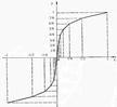A压缩率是指符合下式的对数压缩规律：式中：x为压缩器归一化输入电压；y为压缩器归一化输出电压；A为常数，它决定压缩程度。

A律表示式是一条连续的平滑曲线，用电子线路很难准确地实现。现在由于数字电路技术的发展，这种特性很容易用数字电路来近似实现。13折线特性就是近似于A律的特性。

因为话音信号为交流信号，及输入电压x有正负极性。这就是说在坐标系的第三象限还有对原点奇对称的另一半曲线。第一象限中的第一和第二段折线斜率相同，所以构成一条直线。同样，在第三象限中的第一和第二段折线斜率也相同，并且和第一象限中的斜率相同。所以，这四段折线构成了一条直线。一次，在这正负两个象限中的完整压缩曲线共有13段折线，故称13折线压缩特性。

★增量调制ΔM过载怎样用图标表示：

译码器恢复的信号时阶梯型电压经过低通滤波器平滑后的解调电压。它与编码器输入模拟信号的波形近似，但是存在失真。将这种失真称为量化噪声。这种量化噪声产生的原因有两个。第一个原因是由于编码、译码是用接替波形去近似表示模拟信号波形，有阶梯波形本身的电压突跳产生失真。这是增量调制的基本量化噪声，又称一般量化噪声。它伴随着信号永远存在，即只要有信号，就有这种噪声。

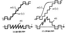第二个原因是信号变化过快引起的失真；这种失真成为过载量化噪声。它发生在输入信号斜率的绝对值过大时。由于当抽样频率和量化台阶一定时，阶梯波的最大可能斜率是一定的。若信号上升的斜率超过阶梯波的最大可能斜率，则阶梯波的上升速度赶不上信号的上升速度，就发生了过载量化噪声。

★分接与复接：P289

复用的目的是为了扩大通信链路的容量，在一条链路上传输多路独立的信号，即实现多路通信。与频分复用相比，时分复用的主要优点是：便于实现数字通信、易于制造、适于采用集成电路实现、成本较低。时分复用的基本原理中的机械旋转开关，在实际电路中是用抽样脉冲取代的。因此，各路抽样脉冲的频率必须严格相同，而且相位也需要有确定的关系，使各路抽样脉冲保持等间隔的距离。在一个多路复用设备中使各路抽样脉冲严格保持这种关系并不难，因为可以有同一时钟提供各种抽样脉冲。

但是随着通信网的发展，时分复用的设备的各路输入信号不再只是单路模拟信号。在通信网同往往有多次复用，有若干链路来的多路时分复用信号，再次复用，构成高次复用信号。这是对于高次复用设备而言，其各路输入信号可能是来自不同地点的多路时分复用信号，并且通常来自各地的输入信号的时钟（频率和相位）之间存在误差。所以在低次群合成高次群时，需要将各路输入信号的时钟调整统一。这种

将低次群合并成高次群的过程成为复接，

将高次群分解为低次群的过程成为分接。

★几种同步：P404

载波同步（载波恢复）

码元同步（时钟同步、时钟恢复、对于二进制码元而言，码元同步又称为位同步。）

群同步  （帧同步、字符同步）

网同步

★集中插入法：P418

    集中插入法又称连贯式插入法。这种方法中采用特殊的群同步码组，集中插入在信息码组的前头，使得接收时能够容易地立即立即捕获它。因此，要求群同步码的自相关特性曲线具有尖锐的单峰，以便容易地从接收码元序列中识别出来。

 

第二篇：通信原理知识点总结

Outline

2012.5

Chapter 0

l  Basic elements of communication systems (p.2)

l  Primary communication resources (p.3)

l  The mobile radio channel (p.18)

l  Block diagram of digital communication system (p.22)

l  Shannon’s information capacity theorem (p.23-24)

Chapter 1

l  Definition and basic concepts of random process

l  Stationary and non-stationary

l  Mean, correlation, and covariance functions, the mean-square value and variance

l  The concept of ergodic process

l  Transmission of a random process through a linear time-invariant filter

n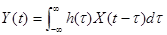 

n  The mean, autocorrelation function, and mean-square value of Y

l  Power spectral density

n  Definition (Equ. 1.38)

n  Input-output relation (Equ. 1.39)

n  Einstein-Wiener-Khintchine relations (Equ. 1.42, 1.43)

n  Properties

l  Gaussian process (Equ. 80)

l  Concept of white noise

l  Representation of narrowband noise

n  The canonical form (Equ. 1.100)

n  Properties of the in-phase and quadrature components (p. 65-66)

n  Representation using envelop and phase components (Equ. 1.105-1.107)

n  Basic concepts of Rayleigh distribution and Rician distribution

l  Uncorrelated and statistically independent (p.58)

n  Uncorrelated: Covariance is 0

n  Statistically independent: defined by joint probability density function

Chapter 2

l  Concepts of amplitude modulation and angle modulation (FM and PM)

l  AM

n  AM signal (Equ. 2.2 and Fig. 2.3), and the amplitude sensitivity k_a

n  Conditions of correct detection (p. 90)

n  Spectrum of AM wave (Equ. 2.5 and Fig. 2.4)

n  Transmission bandwidth B_T = 2W

n  Virtues and limitations of AM

l  Linear modulation schemes

n  The general form (Equ. 2.7)

n  DSB

u  DSB signal (Equ. 2.8 and Fig. 2.5)

u  Spectrum of DSB wave (Equ. 2.9 and Fig. 2.6)

u  Coherent receiver

u  Basic knowledge of costas receiver

u  Basic concept of quadrature-carrier multiplexing

n  Basic concepts of SSB and VSB

l  Concepts of mixer (Fig. 2.16)

l  Concepts of FDM

l  Definitions of angle modulation

l  FM

n  A nonlinear modulation process

n  Single-tone FM modulation

u  Definitions of Df, b

u  Basic knowledge of narrowband and wideband FM

n  Transmission bandwidth

u  Carson’s rule (Equ. 2.55)

u  Know the universal curve

n  Demodulation

u  Frequency demodulation (a direct method) (Fig. 2.30)

u  Know phase-locked loop (an indirect method)

l  Definitions of SNR’s

n  (SNR)_I, (SNR)_O, and (SNR)_C

n  Figure of merit (Equ. 2.81)

l  Comparison of figure of merits between DSB-SC (Equ. 2.88) and AM (Equ. 2.95)

l  Basic concepts of threshold effect of AM (p.138) and FM systems (p.149)

Chapter 3

l  Sampling

n  Definitions of the sampling period and sampling rate

n  Instantaneous sampling and the ideal sampled signal (Equ. 3.1-3.3, Fig. 3.2)

n  Derivation of the interpolation formula (Equ. 3.4-3.9)

n  The sampling theorem and definitions of Nyquist rate and Nyquist interval

n  The methods of combat aliasing effect (p.187)

l  PAM

n  The difference between PAM and natural sampling

n  The concept of “sample and hold”

n  The PAM signal (Equ. 3.10-3.19)

n  The aperture effect

l  Know PPM and PDM

l  Quantization

n  Quantization noise and (SNR)_O of a uniform quantizer (Equ. 3.25-3.33)

l  PCM

n  Basic concepts

u  Discrete in both time and amplitude

u  Sampling, quantizing, and encoding

n  Non-uniform quantizers

u  m-law and A-law

u  Piecewise linear approximation to the companding circuit

n  Five types of line codes and their waveforms

n  Differential encoding

n  Noise in PCM systems

u  Know that noise including channel noise and quantization noise, and that performance is essentially limited by the quantization noise

l  Concepts of TDM (Fig. 3.19)

l  Know the basic concept of digital hierarchy (p.214) and that the basic rate is 64 kbps

l  Concepts of DM and delta-sigma modulation

l  Concepts of linear prediction and linear adaptive prediction

l  DPCM and its processing gain (Equ. 3.82)

Chapter 4

l  Two sources of bit errors: ISI and noise

l  Matched filter

n  Frequency response (Equ. 4.14) and impulse response (Equ. 4.16)

n  Properties: the peak SNR dependents only on signal energy-to-noise psd ratio at the filter input

l  Error rate due to noise

n  Derivation of Equ. 4.35

n  The complementary error function (Equ. 4.29)

n  The result with equiprobable input signals (Equ. 4.38-4.40)

l  The baseband data transmission system model (Fig. 4.7 and Equ. 4.44-4.48)

l  Nyquist’s criterion

n  The Nyquist’s criterion (p.262)

n  The ideal Nyquist channel (Equ. 4.54-4.56 and Fig. 4.8, 4.9)

n  Raised cosine spectrum (Equ. 4.59, Fig. 4.10)

u  The definition of a and the bandwidth B_T

l  Correlative-level coding (partial response signaling)

n  Duobinary signaling (class I partial response)

u  Basic concepts (Fig. 4.11, 4.13, Equ. 4.66, 4.71)

u  The concept of decision feedback

u  Error-propagation and precoding

n  Generalized form of correlative-level coding

l  Baseband M-ary PAM transmission (Equ. 4.84)

l  ADSL (Fig. 4.26)

l  Optimum linear receiver

n  For linear channel with both ISI and noise

n  The MMSE receiver (Equ. 4.110 and Fig. 4.27)

l  Adaptive equalization

n  The LMS algorithm (Equ. 4.114, 4.115)

n  The basic concept of decision-feedback equalization (Fig. 4.32)

Chapter 5

l  Geometric representation of signals (Equ. 5.5-5.7 and Fig. 5.3)

n  The vector form (Equ. 5.8) and definitions of length, Euclidean distance, and angle

n  Gram-Schmidt orthogonalization procedure

l  Conversion of the continuous AWGN channel into a vector channel

n  Basic formulations (Equ. 5.28-5.34)

n  The vector representation represents sufficient statistics for detection

l  Log-likelyhood functions for AWGN channel (Equ. 5.51)

l  Maximum likelihood decoding

n  The concept of signal constellation

n  The maximum likelihood rule (Equ. 5.55), for AWGN channel, the rule is Equ. 5.59 and 5.61

l  Equivalence of correlation and matched filter sampled at time T

l  Probability of error

n  Know the invariance to rotation and translation

n  The concept of the minimum energy signals

n  Know how to use union bound to derive a upper bound (p. 332 – 335) (Equ. 5.89)

n  Know that there is, in general, no unique relationships between symbol error probabilities and BER

Chapter 6

l  Basic concepts of keying and ASK, FSK, and PSK

l  The relationship between baseband and passband power spectral density (Equ. 6.4)

l  Bandwidth efficiency (Equ. 6.5)

l  The passband transmission model

l  Coherent PSK

n  BPSK

u  Basic definitions (Equ. 6.8-6.14, Fig. 6.3)

u  Error probability (Equ. 6.20)

n  QPSK

u  Basic definitions (Equ. 6.23-6.27)

u  Error probability (Equ. 6.34, 6.38)

u  Generation and detection (Fig. 6.8)

n  M-PSK

u  Basic definitions (Equ. 6.46)

u  Bandwidth efficiency

u  Know that the power spectra of M-PSK has no discrete frequency component

l  M-QAM

n  Basic definitions (Equ. 6.53-6.55)

n  QAM square constellations (Fig. 6.17)

l  Coherent FSK

n  Coherent BFSK

u  Basic definitions (Sunde’s FSK) (Equ. 6.86-6.91, Fig. 6.25)

u  Error probability (Equ. 6.102)

u  Know that the power spectra of BFSK has discrete frequency components

n  MSK

u  The concept of CPFSK

u  The concept of MSK

u  The phase trellis

u  Signal-space diagram (Fig. 6.29)

u  Error probability (Equ. 6.127)

n  Bandwidth efficiency of M-FSK signals

l  Noncoherent receivers (Fig. 6.37)

l  The reason of envelop detection (Fig. 6.38)

l  Error probability of noncoherent receiver (Equ. 6.163)

l  Noncoherent BFSK

n  Receiver structure (Fig. 6.42)

n  Error probability (Equ. 6.181)

l  DPSK

n  Basic concepts (Fig. 6.43, 6.44)

n  Error probability (Equ. 6.184)

l  Comparison of digital modulation schemes

n  Relationship among the error probabilities (Table 6.8 and Fig. 6.45)

n  Bandwidth efficiencies of M-PSK, M-QAM, and M-FSK