********************************

《信号分析与处理》

实 验 报 告

实验名称：信号产生 班 级：电气研-14 学 号：2014312080114 姓 名：刘家利 联系方式：136xxxxxxxx

一． 实验内容：

1. 产生至少三种典型连续信号， 三种典型离散序列（自选）。

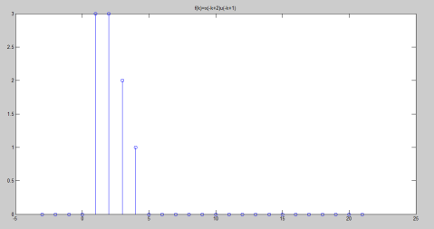
2. 绘制图形，在同一张图中出现两种时间连续信号， 两种时间离散信号。分别标注横纵坐标， 各信号名称。 图名为“信号的产生—本人姓名” 3. 已知信号 x[k]?[0,0,1,2,3,3,3,3,3,0]?4?k?5，编写程序 f(k)?x(?k?2)?(?k?1) ，计算并绘制f(k)并确定其长度。（ 其中 ?(k)为单位冲激信号）

二． 实验方案：

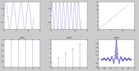
1. （1）利用subplot函数将窗口分割为六个小窗口即 2x3。

（2）利用plot函数将函数图行描出。

（3）利用stem函数将函数图行离散化。

（4） 利用title对函数标题。

2. （1）定义自变量的范围，很重要，不同的函数变化快慢不

一样，这样不同曲线幅值相差很大，看起来不明显。

（2）定义四个函数。

（3）利用stem函数将函数图行离散化。

（4）利用xlabel，title，legend对函数标注，标题，注释。

3. （1）根据要求先对函数平移取反求得f（-k+2）。

（2）求得u（k）函数并求得u（-k+1）。

（3）确定相乘后n的大小即自变量范围，然后相乘。

（4）利用xlabel，title，legend对函数标注，标题，注释。

三． 仿真结果分析总结

实验图形一

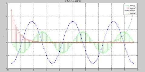
实验图形二

实验图形三

总结：对于两离散序列的乘积，实验结果与理论分析一致。对于本题3的离散序列相乘需要平移，反褶，求得相应的序列再相乘，而序列的相乘需要先确定自变量n的范围然后矩阵相乘。对于实验1,2学会了title，legend，还有stem函数的使用。

附录.

1. 源程序及说明一

x=0:0.1:4*pi; % 定义x的范围及步长 subplot(2, 3, 1); plot(x, sin(2*x)); % 一个窗口分割成6个图形，此为11图形 subplot(2, 3, 2); plot(x, sin(4*x)); % 一个窗口分割成6个图形，此为12图形 subplot(2, 3, 3); plot(x, x); % 一个窗口分割成6个图形，此为13图形 n1=0:5;y1=[1,1,1,1,1,1];

subplot(2, 3, 4); stem(n1,y1);

title('y1序列'); % 一个窗口分割成6个图形，此为21图形 n2=0:5;y2=[1,2,3,4,5,6];

subplot(2, 3, 5); stem(n1,y2); % stem为离散化函数 title('y2序列'); % 一个窗口分割成6个图形，此为22图形 n3=-8*pi:0.5:8*pi;y3=1*(sin(n3)./n3); subplot(2, 3, 6);stem(n3,y3);

title('y3序列'); % 一个窗口分割成6个图形，此为23图形

2．源程序及说明二

x=-3*pi:0.2:3*pi; % 定义x的范围及步长 y1=4*sin(x); % 定义函数的y1,y2,y3,y4. y2=0.001*exp(-x);

y3=8*cos(x);

y4=0.001*exp(x);

stem(x,y1,'g'); % 离散化函数的y1 hold on

stem(x,y2,'r'); % 离散化函数的y2 hold on

plot(x,y3,'--*',x,y4); % 离散化函数的y3 xlabel('x'); %写出x坐标标示 ylabel('y'); %写出y坐标标示 title('信号的产生-刘家利'); %写出此图形代表标题 legend('4sin(x)','0.001e^{-x}','8cos(x)','0.001e^{x}'); grid on %绘上网格

3. 源程序及说明三

n5=-4:5; % 已知n5的范围 x=[0,0,1,2,3,3,3,3,3,0]; % 已知x的值 x11=fliplr(x);n11=-fliplr(n5); % 做反褶变换

n12=n11+2; x12=x11; % 做平移变换

n0=0:20; % 定义单位阶跃序列的范围，理论上inf大这里取20 u=ones(1,length(n0)); % 定义单位阶跃序列 x14=fliplr(u);n14=-fliplr(n0); % 单位阶跃反褶 n15=n0+1; x15=x14; % 单位阶跃平移

n=min(min(n12),min(n15)):max(max(n15),max(n12)); % 确定n范围 y1=zeros(1,length(n));y2=y1; %定义两个零矩阵 y1(find((n>=min(n12))&(n<=max(n12))==1))=x12; y2(find((n>=min(n15))&(n<=max(n15))==1))=x15; y=y1.*y2;

subplot(1,1,1),stem(n,y);title('f(k)=x(-k+2)u(-k+1)'); %对两个零矩阵赋值 %对两个零矩阵相乘操作 %matlab输出相乘后的序列

 

第二篇：数字信号实验报告1

数字信号处理导论实验报告

                        姓名：金涛

                        学号：201005090209

实验一   信号、系统及系统响应

当系统的输入输出差分方程为：

        Y(n)-0.8y(n-1)-0.5y(n-2)=0.7x(n)+0.3x（n-1）

通过 MATLAB 编程实现并考虑如下问题：

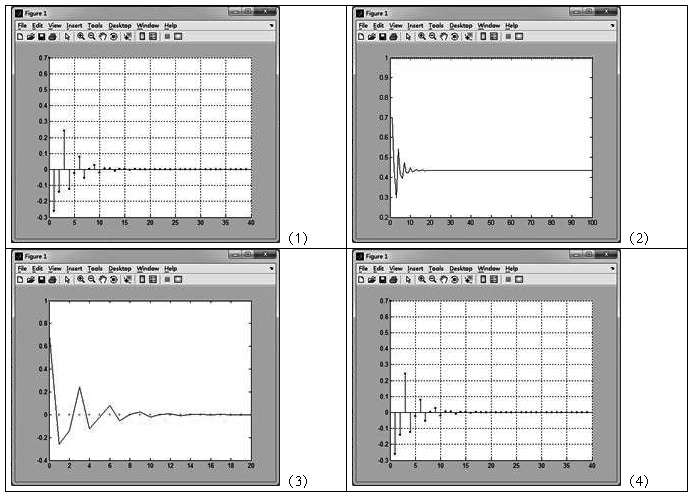
（1）当系统的输入为单位冲激函数时，分别利用filter 函数和impz 函数得到的系统单位冲激响应曲线。

（2）当系统的输入为单位阶跃函数时，分别利用filter 函数和impz 函数得到的系统单位阶跃响应曲线。

（3）对于不同的输入，系统的输出有什么变化，试讨论之。

（一）实验原理

对一个给定的LSI系统，其转移函数H(z)的定义和表示形式为：.  习惯上，令H(z)=B(z)/A(z).在MATLAB中，因为数组的下标不能为零（当然也不能为负值），因此，可重新表示为  H(z)=

在有关MATLAB的系统分析的文件中。分子和分母的系数被定义为向量，即

b=[b(1),b(2),b(3),...,b(+1)]

a=[a(1),a(2),...,a()]

并要求a（1）=1，如果a(1)≠1,则程序自动将其规划为1

（二）实验内容

源程序

x=ones(100);t=1:100;   %产生单位阶跃序列

b=[.7,.3];              %b向量

a=[1,.8,.5];             %a向量

y=filter(b,a,x);          %实现实验1 ，图（1）

plot(t,x,'g.',t,y,'k-');

[h,t]=impz(b,a,40);       %求出单位抽样响应。图（2）

stem(t,h,'.');grid on;

t=0:20;

 x=[1,zeros(1,20)];    %产生单位采样序列

 b=[.7,.3];             %形成b向量

 a=[1,.8,.5];            %形成a向量       

 y=filter(b,a,x);         %filter函数  图（3）

 plot(t,x,'g.',t,y,'k-');

 t=0:20;

 x=[1,zeros(1,20)];

 b=[.7,.3];

 a=[1,.8,.5];

[h,t]=impz(b,a,40);  %impz函数 图（4）

 stem(t,h,'.');grid on;

（三）实验结果

（四）分析结果

输入为离散是，输出为连续。相反，输入为连续，输出为离散。

对于单位阶跃和单位抽样输入来说，输出没有变化

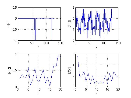
实验二使用FFT作频谱分析

（1） 使用FFT 对MATLAB 中的数据noissin.dat 进行谱分析。

（2） 使用FFT 对语音数据noisyspeech.wav 进行谱分析。

（一）实验原理

（1）离散傅里叶变换(DFT)公式为：

X(k)=∑x(n)W^nk;

x(n)=∑X(k)W^-nk;

其中w=e^(2∏nk/N),N为离散序列的长度。

（2）快速傅里叶变换(FFT)是利用w因子的取值特点，减少DFT的复数乘法的次数。其中一种是时间抽取基2算法，它将时间按奇偶逐级分开，直到两点的DFT。MATLAB提供了fft函数可用于计算FFT，器调用形式为;X=fft（x）或X=fft（x，N），N为2的整数次幂，若x的长度小于N，则补零，若超过则舍去N后的数据。

（3）函数形式[y,fs,bits]=wavread('Blip',[N1 N2]);用于读取语音，采样值放在向量y中，fs表示采样频率(Hz)，bits表示采样位数。[N1 N2]表示读取从N1点到N2点的值（若只有一个N的点则表示读取前N点的采样值）。

函数形式s=noissin（n1，n2）用于读取MALAB的噪声信号。

（二）实验内容

xx=wavread('noisyspeech.wav');

fs=100;N=128;

x=xx(1:N);

n=1:N;

X=abs(fft(x,N));

subplot(221);plot(n,x);

xlabel('n');ylabel('x(n)');

grid on;

subplot(222);plot(n,X);

xlabel('k');ylabel('|X(k)|');

grid on;

load noissin;

s=noissin(1:20);

S=fft(s);

subplot(223);plot(abs(s));

xlabel('n');ylabel('|s(n)|');

grid on;

subplot(224);plot(abs(S));

xlabel('k');ylabel('|S(k)|');

grid on;

（三）实验结果及分析

实验三  使用双线性Z变换设计IIR滤波器

使用双线性Z 变换法设计一个低通数字IIR 滤波器，给定的数字滤波器的技术指标为fp=100Hz,fs=300Hz,ap=3dB,as=20dB,抽样频率Fs=1000Hz

（一）实验原理

1）设计滤波器就是要设计一个系统是其能让一定频率的波段通过或滤去，对IIR滤波器，器转移函数是：H(Z)=(∑bz^(-r))/(1+∑az^(-k))。

（2）设计的一般原则：若使滤波器拒绝某个频率，应在单位园上相应的频率处设置一个零点，反之则设置一个极点。

(3)低通数字IIR滤波器设计步骤：

给出数字低通滤波器的技术要求→映射为模拟低通的技术要求→归一化为模拟低通滤波器的技术要求→设计出G(P)→G(S)→映射到数字滤波器的转移函数G(Z)。

(3)双线性Z变换，即S平面到Z平面的映射关系：S=2（Z-1）/Ts（Z+1）。

（二）实验内容

fp=100;fs=300;Fs=1000; %给定要设计的低通滤波器的设计频率；

rp=3;rs=20; %给定需要的衰减，单位为db；

wp=2*pi*fp/Fs;

ws=2*pi*fs/Fs;Fs=Fs/Fs; %令Fs=1

wap=tan(wp/2);was=tan(ws/2); %实现由数字滤波器到模拟滤波器的转换；

[n,wn]=buttord(wap,was,rp,rs,'s'); %求模拟滤波器的阶次；

[z,p,k]=buttap(n);  %设计模拟低通巴特沃斯滤波器。得到极零点；

[bp,ap]=zp2tf(z,p,k);  %由极零点得到滤波器分子分母多项式的系数；

[bs,as]=lp2lp(bp,ap,wap);  %归一化低通到实际低通的转换；

[bz,az]=bilinear(bs,as,Fs/2);  %实现s到z的转换；

[h,w]=freqz(bz,az,256,Fs*1000);  %求出滤波器的频率响应；

plot(w,abs(h));grid on;

（三）实验结果

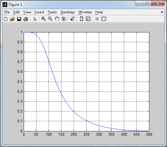
（四）结果分析

由图可知，数字滤波器的幅频曲线完全满足技术要求，而且在f>fp后，数字滤波器的幅频响应的衰减比较快，这正是我们希望的

实验四  窗函数法设计FIR数字滤波器

根据下列指标，设计一个FIR数字低通滤波器：ω=2.0∏，ω=4.0∏

Ap=0.25dB，As=50dB。

（1） 分别考查矩形窗、三角窗、Hanning窗、Hamming窗并分析这些不同的窗函数对滤波器的幅度响应有什么影响。

（2） 选择一个合适的窗函数，确定单位冲激响应，绘出所设计的滤波器的幅度响应。

（一）实验目的：了解常用的几种窗函数，能正确选择适当的窗函数进行滤波器设计；掌握窗函数法设计数字低通滤波器。

（二）实验原理

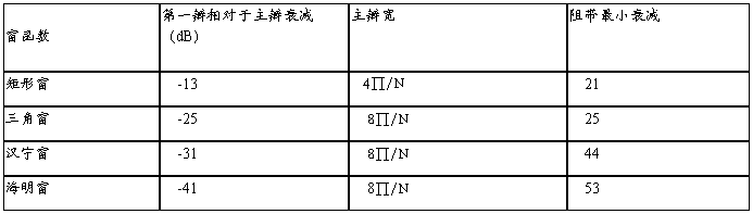
常用的窗函数：

1、矩形窗 函数为boxcar和rectwin，调用格式：

        w= boxcar（N） w= rectwin(N)

其中N是窗函数的长度，返回值w是一个N阶的向量。

2、三角窗 函数为triang，调用格式：

        w= triang(N)

3、汉宁窗 函数为hann，调用格式：

        w= hann（N）

4、海明窗 函数为hamming，调用格式：

       w= hamming（N）

各个窗函数的性能比较

（三）实验内容

1、题一：生成四种窗函数。

矩形窗、三角窗、汉宁窗、海明窗，并观察其频率响应。

源程序：

clear all ;

n=20;

window=rectwin(n);

[h,w]=freqz(window,1);

subplot(4,2,1);

stem(window);

title('矩形窗');

subplot(4,2,2);

plot(w/pi,20*log(abs(h))/abs(h(1)));

title('矩形窗的频率响应');

hold on;

window=triang(n);

[h,w]=freqz(window,1);

subplot(4,2,3);

stem(window);

title('三角窗');

subplot(4,2,4);

plot(w/pi,20*log(abs(h))/abs(h(1)));

title('三角窗的频率响应');

hold on;

window=hann(n);

[h,w]=freqz(window,1);

subplot(4,2,5);

stem(window);

title('汉宁窗');

subplot(4,2,6);

plot(w/pi,20*log(abs(h))/abs(h(1)));

title('汉宁窗的频率响应');

hold on;

window=hamming(n);

[h,w]=freqz(window,1);

subplot(4,2,7);

stem(window);

title('海明窗');

subplot(4,2,8);

plot(w/pi,20*log(abs(h))/abs(h(1)));

title('海明窗的频率响应');

hold on;

实验结果：

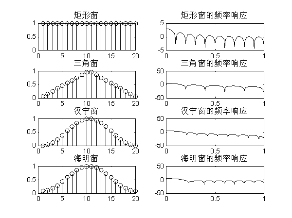
分析实验结果：

通过对窗函数的调用，使4个窗函数的时域及频域图放置在一起，比较直观地看出各个窗函数的特性。

2、题二：根据下列技术指标，设计一个FIR数字低通滤波器：wp=0.2π，ws=0.4π，ap=0.25dB， as=50dB，选择一个适当的窗函数，确定单位冲激响应，绘出所设计的滤波器的幅度响应。

提示：根据窗函数最小阻带衰减的特性表，可采用海明窗可提供大于50dB的衰减，其过渡带为6.6π/N，因此具有较小的阶次。

源程序：

clear all;

wp=0.2*pi;                        %通带截止频率   

ws=0.4*pi;                        %阻带截止频率

tr_wdith=ws-wp;                   %过渡带宽度

N=ceil(6.6*pi/tr_wdith)+1;           %得到N

n=0:1:N-1;

wc=(ws+wp)/2;                    %理想低通滤波器的截止频率

hd=ideal_lp1(wc,N);                %理想低通滤波器的单位冲激响应

w_ham=(hamming(N))';             %海明窗

h=hd.*w_ham;                     %截取得到实际的单位脉冲响应

[db,mag,pha,w]=freqz_m2(h,1);       %计算实际滤波器的幅度响应

subplot(221);

stem(n,hd,'k');

title('理想低通滤波器的单位脉冲响应hd（n）');

subplot(222);

stem(n,w_ham,'k');

title('海明窗w（n）');

subplot(223);

stem(n,h,'k');

title('实际低通滤波器的单位脉冲响应h（n）');

subplot(224);

plot(w/pi,db,'k');

title('实际低通滤波器的幅度响应（dB）');

axis([0,1,-100,10]);

子函数freqz_m2(b,a)：

function[db,mag,pha,w]=freqz_m2(b,a);

%滤波器的幅值响应（相对、绝对）、相位响应

%db：相对幅值响应；

%mag：绝对幅值响应；

%pha：相位响应；

%w：采样频率；

%b:系统函数H（Z）的分子项（对FIR,b=h）;

%a:系统函数H（Z）的分母项（对FIR,a=1）;

[H,w]=freqz(b,a,1000,'whole');

H=(H(1:1:501))';

w=(w(1:1:501))';

mag=abs(H);

db=20*log10((mag+eps)/max(mag));

pha=angle(H)

子函数ideal_lp1(wc,N)：

function hd=ideal_lp1(wc,N);

alpha=(N-1)/2;

n=0:1:N-1;

m=n-alpha+eps;

hd=sin(wc*m)./(pi*m);

实验结果：

分析实验结果：

用窗函数的方法设计FIR低通数字滤波器，其性能十分逼近与理想的IIR数字低通滤波器，并且具有较好的衰减特性。如图所示。

实验五用C++编程实现FFT并作频分析

（一）源程序

#include <stdio.h>

#include <stdlib.h>

#include <math.h>

const int N = 1024;

const float PI = 3.1416;

inline void swap (float &a, float &b)

{

    float t;

    t = a;

    a = b;

    b = t;

}

void bitrp (float xreal [], float ximag [], int n)

{

    // 位反转置换 Bit-reversal Permutation

    int i, j, a, b, p;

    for (i = 1, p = 0; i < n; i *= 2)

        {

        p ++;

        }

    for (i = 0; i < n; i ++)

        {

        a = i;

        b = 0;

        for (j = 0; j < p; j ++)

            {

            b = (b << 1) + (a & 1);    // b = b * 2 + a % 2;

            a >>= 1;        // a = a / 2;

            }

        if ( b > i)

            {

            swap (xreal [i], xreal [b]);

            swap (ximag [i], ximag [b]);

            }

        }

}

void FFT(float xreal [], float ximag [], int n)

{

    // 快速傅立叶变换，将复数 x 变换后仍保存在 x 中，xreal, ximag 分别是 x 的实部和虚部

    float wreal [N / 2], wimag [N / 2], treal, timag, ureal, uimag, arg;

    int m, k, j, t, index1, index2;

   

    bitrp (xreal, ximag, n);

    // 计算 1 的前 n / 2 个 n 次方根的共轭复数 W'j = wreal [j] + i * wimag [j] , j = 0, 1, ... , n / 2 - 1

    arg = - 2 * PI / n;

    treal = cos (arg);

    timag = sin (arg);

    wreal [0] = 1.0;

    wimag [0] = 0.0;

    for (j = 1; j < n / 2; j ++)

        {

        wreal [j] = wreal [j - 1] * treal - wimag [j - 1] * timag;

        wimag [j] = wreal [j - 1] * timag + wimag [j - 1] * treal;

        }

    for (m = 2; m <= n; m *= 2)

        {

        for (k = 0; k < n; k += m)

            {

            for (j = 0; j < m / 2; j ++)

                {

                index1 = k + j;

                index2 = index1 + m / 2;

                t = n * j / m;    // 旋转因子 w 的实部在 wreal [] 中的下标为 t

                treal = wreal [t] * xreal [index2] - wimag [t] * ximag [index2];

                timag = wreal [t] * ximag [index2] + wimag [t] * xreal [index2];

                ureal = xreal [index1];

                uimag = ximag [index1];

                xreal [index1] = ureal + treal;

                ximag [index1] = uimag + timag;

                xreal [index2] = ureal - treal;

                ximag [index2] = uimag - timag;

                }

            }

        }

}

void  IFFT (float xreal [], float ximag [], int n)

{

    // 快速傅立叶逆变换

    float wreal [N / 2], wimag [N / 2], treal, timag, ureal, uimag, arg;

    int m, k, j, t, index1, index2;

   

    bitrp (xreal, ximag, n);

    // 计算 1 的前 n / 2 个 n 次方根 Wj = wreal [j] + i * wimag [j] , j = 0, 1, ... , n / 2 - 1

    arg = 2 * PI / n;

    treal = cos (arg);

    timag = sin (arg);

    wreal [0] = 1.0;

    wimag [0] = 0.0;

    for (j = 1; j < n / 2; j ++)

        {

        wreal [j] = wreal [j - 1] * treal - wimag [j - 1] * timag;

        wimag [j] = wreal [j - 1] * timag + wimag [j - 1] * treal;

        }

    for (m = 2; m <= n; m *= 2)

        {

        for (k = 0; k < n; k += m)

            {

            for (j = 0; j < m / 2; j ++)

                {

                index1 = k + j;

                index2 = index1 + m / 2;

                t = n * j / m;    // 旋转因子 w 的实部在 wreal [] 中的下标为 t

                treal = wreal [t] * xreal [index2] - wimag [t] * ximag [index2];

                timag = wreal [t] * ximag [index2] + wimag [t] * xreal [index2];

                ureal = xreal [index1];

                uimag = ximag [index1];

                xreal [index1] = ureal + treal;

                ximag [index1] = uimag + timag;

                xreal [index2] = ureal - treal;

                ximag [index2] = uimag - timag;

                }

            }

        }

    for (j=0; j < n; j ++)

        {

        xreal [j] /= n;

        ximag [j] /= n;

        }

}

void FFT_test ()

{

    char inputfile [] = "input.txt";    // 从文件 input.txt 中读入原始数据

    char outputfile [] = "output.txt";    // 将结果输出到文件 output.txt 中

    float xreal [N] = {}, ximag [N] = {};

    int n, i;

    FILE *input, *output;

    if (!(input = fopen (inputfile, "r")))

        {

        printf ("Cannot open file. ");

        exit (1);

        }

    if (!(output = fopen (outputfile, "w")))

        {

        printf ("Cannot open file. ");

        exit (1);

        }

       

    i = 0;

    while ((fscanf (input, "%f%f", xreal + i, ximag + i)) != EOF)

        {

        i ++;

        }

    n = i;    // 要求 n 为 2 的整数幂

    while (i > 1)

        {

        if (i % 2)

            {

            fprintf (output, "%d is not a power of 2! ", n);

            exit (1);

            }

        i /= 2;

        }

    FFT (xreal, ximag, n);

    fprintf (output, "FFT:    i     real imag ");

    for (i = 0; i < n; i ++)

        {

        fprintf (output, "%4d    %8.4f    %8.4f ", i, xreal [i], ximag [i]);

        }

    fprintf (output, "================================= ");

    IFFT (xreal, ximag, n);

    fprintf (output, "IFFT:    i     real imag ");

    for (i = 0; i < n; i ++)

        {

        fprintf (output, "%4d    %8.4f    %8.4f ", i, xreal [i], ximag [i]);

        }

    if ( fclose (input))

        {

        printf ("File close error. ");

        exit (1);

        }

    if ( fclose (output))

        {

        printf ("File close error. ");

        exit (1);

        }

}

int main ()

{

    FFT_test ();

    return 0;

}

（二）实验结果

/**************************************************

////////////////////////////////////////////////
// sample: input.txt
////////////////////////////////////////////////

 0.5751 0
 0.4514 0
 0.0439 0
 0.0272 0
 0.3127 0
 0.0129 0
 0.3840 0
 0.6831 0
 0.0928 0
 0.0353 0
 0.6124 0
 0.6085 0
 0.0158 0
 0.0164 0
 0.1901 0
 0.5869 0

////////////////////////////////////////////////
// sample: output.txt
////////////////////////////////////////////////
FFT:
 i real imag
 0 4.6485 0.0000
 1 0.0176 0.3122
 2 1.1114 0.0429
 3 1.6776 -0.1353
 4 -0.2340 1.3897
 5 0.3652 -1.2589
 6 -0.4325 0.2073
 7 -0.1312 0.3763
 8 -0.1949 0.0000
 9 -0.1312 -0.3763
 10 -0.4326 -0.2073
 11 0.3652 1.2589
 12 -0.2340 -1.3897
 13 1.6776 0.1353
 14 1.1113 -0.0429
 15 0.0176 -0.3122
=================================
IFFT:
 i real imag
 0 0.5751 -0.0000
 1 0.4514 0.0000
 2 0.0439 -0.0000
 3 0.0272 -0.0000
 4 0.3127 -0.0000
 5 0.0129 -0.0000
 6 0.3840 -0.0000
 7 0.6831 0.0000
 8 0.0928 0.0000
 9 0.0353 -0.0000
 10 0.6124 0.0000
 11 0.6085 0.0000
 12 0.0158 0.0000
 13 0.0164 0.0000
 14 0.1901 0.0000
 15 0.5869 -0.0000


**************************************************/