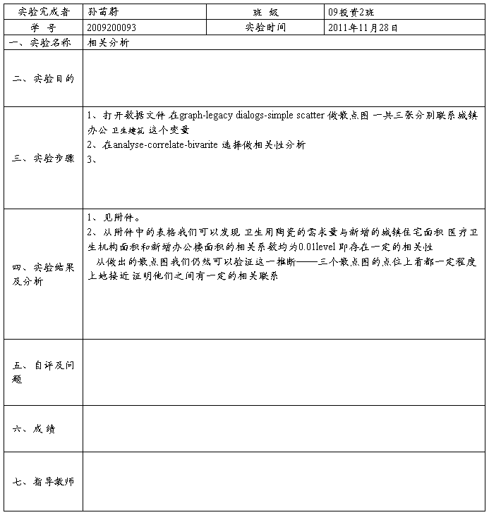
实验报告(相关分析)
《经济分析方法与手段》实验分析报告
附件一、
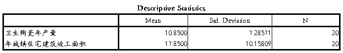
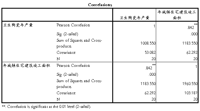
1 陶瓷产量与城镇住宅建筑面积的相关分析
散点图


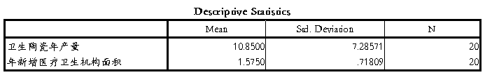
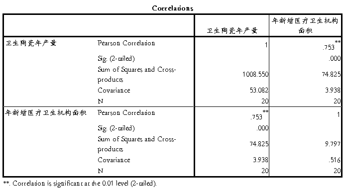
2 与新增医疗卫生机构面积的关系
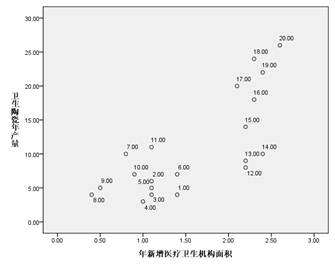
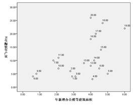
3 与新增办公楼面积的关系
附件二、
说明:如果实验分析需要用到SPSS的图表,依次在附件中列出,并在“实验结果及分析”中相应说明。
第二篇:实验报告9 典型相关分析
实验九 典型相关分析
实验目的和要求
能利用原始数据与相关矩阵、协主差矩阵作相关分析,能根据SAS输出结果选出满足要求的几个典型变量.
实验要求:编写程序,结果分析.
实验内容:4.9
方法一:SAS
data examp4_9;
input x1-x2 y1-y2;
cards;
191 155 179 145
195 149 201 152
181 148 185 149
183 153 188 149
176 144 171 142
208 157 192 152
189 150 190 149
197 159 189 152
188 152 197 159
192 150 187 151
179 158 186 148
183 147 174 147
174 150 185 152
190 159 195 157
188 151 187 158
163 137 161 130
195 155 183 158
186 153 173 148
181 145 182 146
175 140 165 137
192 154 185 152
174 143 178 147
176 139 176 143
197 167 200 158
190163187150;
run;
proccancorr data=examp4_9 corr;
var x1-x2;
with y1-y2;
run;
The SAS System 16:48 Sunday, October 31, 2012 1
The CANCORR Procedure
Correlations Among the Original Variables
Correlations Among the VAR Variables(变量x1-x2的相关系数矩阵 )
)
x1 x2
x1 1.0000 0.7504
x2 0.7504 1.0000
Correlations Among the WITH Variables(变量y1-y2的相关系数矩阵 )
)
y1 y2
y1 1.0000 0.8397
y2 0.8397 1.0000
Correlations Between the VAR Variables and the WITH Variables
变量x1-x3与y1-y3的相关系数矩阵
y1 y2
x1 0.7092 0.7050
x2 0.7140 0.7440
The SAS System 16:48 Sunday, October 31, 2012 2
The CANCORR Procedure
Canonical Correlation Analysis
Adjusted Approximate Squared
Canonical Canonical Standard Canonical
Correlation Correlation Error Correlation
1  0.801420 0.788167 0.074591
  0.642274
2  0.084522 . 0.207025
  0.007144
Test of H0: The canonical correlations in the
Eigenvalues of Inv(E)*H current row and all that follow are zero
= CanRsq/(1-CanRsq)
Likelihood Approximate
Eigenvalue Difference Proportion Cumulative Ratio F Value Num DF Den DF Pr > F
1 1.7954 1.7882 0.9960 0.9960 0.35517013 6.78 4 40 0.0003
2 0.0072 0.0040 1.0000 0.99285597 0.15 1 21 0.7014
检验假设
检验统计量 ,
, 为第一、第二自由度.由检验结果可知,
 ,.故只有第一对典型变量显著相关.取第一对进行分析即可.
Multivariate Statistics and F Approximations
S=2 M=-0.5 N=9
Statistic Value F Value Num DF Den DF Pr > F
Wilks' Lambda 0.35517013 6.78 4 40 0.0003
Pillai's Trace 0.64941830 5.05 4 42 0.0021
Hotelling-Lawley Trace 1.80263313 8.88 4 23 0.0002
Roy's Greatest Root 1.79543769 18.85 2 21 <.0001
NOTE: F Statistic for Roy's Greatest Root is an upper bound.
NOTE: F Statistic for Wilks' Lambda is exact.
The SAS System 16:48 Sunday, October 31, 2012 3
The CANCORR Procedure
Canonical Correlation Analysis
Raw Canonical Coefficients for the VAR Variables
V1 V2
x1 0.0474933802 -0.144760311
x2 0.0840477791 0.1959848929
Raw Canonical Coefficients for the WITH Variables
W1 W2
y1 0.0448783575 -0.174269545
y2 0.0850389917 0.2549589923
数据未标准化结果,即利用协方差矩阵分析的结果


The SAS System 16:48 Sunday, October 31, 2012 4
The CANCORR Procedure
Canonical Correlation Analysis
Standardized Canonical Coefficients for the VAR Variables
V1 V2
x1 0.4716 -1.4375
x2 0.5963 1.3904
Standardized Canonical Coefficients for the WITH Variables
W1 W2
y1 0.4593 -1.7835
y2 0.5827 1.7471
 ,
, .
.
第一对典型变量


The SAS System 16:48 Sunday, October 31, 2012 5
The CANCORR Procedure
Canonical Structure
Correlations Between the VAR Variables and Their Canonical Variables
V1 V2
x1 0.9191 -0.3941
x2 0.9502 0.3117
Correlations Between the WITH Variables and Their Canonical Variables
W1 W2
y1 0.9486 -0.3164
y2 0.9684 0.2494
Correlations Between the VAR Variables and the Canonical Variables of the WITH Variables
W1 W2
x1 0.7365 -0.0333
x2 0.7615 0.0263
Correlations Between the WITH Variables and the Canonical Variables of the VAR Variables
V1 V2
y1 0.7602 -0.0267
y2 0.7761 0.0211
原变量和第一对变量相关程度高,后一组提取的信息很少,与典型对系数一致。
方法二:MATLAB
>> a=[data];
[n,m]=size(a);
b=a./(ones(n,1)*std(a));
R=cov(b);
X=b(:,1:2);
Y=b(:,3:4);
[A,B,r,U,V,ststs]=canoncorr(X,Y)
A =
0.5522 -1.3664
0.5215 1.3784
B =
0.5044 -1.7686
0.5383 1.7586
r =
0.7885 0.0537
U =
0.5731 -0.0137
0.3750 -1.6953
-0.4877 0.0774
-0.0209 0.7322
-1.0535 0.0294
1.6762 -2.0193
0.1063 -0.6685
1.1955 -0.1057
0.1912 -0.1546
0.2760 -1.0884
0.1065 2.2268
-0.4453 -0.3895
-0.7422 1.4311
0.7995 0.8741
0.1205 -0.3416
-2.2840 0.5404
0.7994 -0.5736
0.1488 0.3123
-0.6999 -0.4835
-1.3930 -0.5784
0.5590 -0.3406
-1.2373 0.1224
-1.4072 -0.9053
1.7614 1.3899
1.0825 1.6219
V =
-0.5833 -0.2587
1.0836 -2.2993
0.0390 -0.2672
0.1898 -0.7957
-1.2259 0.3643
0.6314 -0.7140
0.2902 -1.1480
0.4807 -0.1856
1.4442 0.2398
0.3000 -0.0954
0.0090 -0.7055
-0.6741 1.1462
0.2797 0.5190
1.1832 0.0680
0.8615 1.7392
-2.6910 -1.0193
0.6605 2.4438
-0.6441 1.5845
-0.3524 -0.5250
-1.9285 0.1107
0.2797 0.5190
-0.4731 0.4416
-0.8945 -0.2544
1.5147 -0.5507
0.2197 -0.3574
ststs =
Wilks: [0.3772 0.9971]
df1: [4 1]
df2: [42 22]
F: [6.5972 0.0637]
pF: [3.2565e-004 0.8031]
chisq: [20.9642 0.0639]
pChisq: [3.2189e-004 0.8004]
dfe: [4 1]
p: [3.2189e-004 0.8004]
-
现代实验分析报告
水泥中MgOCaOAl2O3Fe2O3含量的测定一实验目的1学习复杂物质分析的方法2掌握尿素均匀沉淀法二实验原理本实验采用硅酸盐水…
-
实验结果分析报告
1亚硝酸钠测定结果标准液质量与吸光度表亚硝酸钠标准液质量000123457510125吸光度0002600430068005701…
-
实验报告 范本
研究生实验报告范本实验课程实验名称实验地点学生姓名学号指导教师范本实验时间年月日一实验目的熟悉电阻型气体传感器结构及工作原理进行基…
-
程序分析实验报告
程序分析第二次实验报告13091372代树理开发环境语言java编译器myeclipse操作系统windowsXP另外使用的ANT…
-
实验报告(相关分析)
经济分析方法与手段实验分析报告附件一1陶瓷产量与城镇住宅建筑面积的相关分析散点图2与新增医疗卫生机构面积的关系3与新增办公楼面积的…
-
有关实验报告的书写格式
有关实验报告的书写格式江苏省泗阳县李口中学沈正中一、完整实验报告的书写完整的一份实验报告一般包括以下项目:实验名称:实验目的:实验…
-
实验报告 范本
研究生实验报告范本实验课程实验名称实验地点学生姓名学号指导教师范本实验时间年月日一实验目的熟悉电阻型气体传感器结构及工作原理进行基…
-
分析化学实验报告(武汉大学第五版)
分析化学实验报告陈峻贵州大学矿业学院贵州花溪550025摘要熟悉电子天平的原理和使用规则同时可以学习电子天平的基本操作和常用称量方…
-
语法分析实验报告(实验二)
编译原理语法分析实验报告软工082班兰洁20xx31104044一实验内容二实验目的三实验要求四程序流程图主函数scannerir…
-
股票基本面分析实验报告
《证券投资理论与实务》实验报告实验项目名称:ST大荒股票基本分析学生姓名:**专业:13金融学专升本学号:****实验地点:C34…
-
化学实验研究报告
?化学实验研究报告我们初三学习了一个学期的化学,从中学到了很多有趣的知识,初步学会了用简单的仪器和药品进行实验的方法,同时也对化学…